Note on Classical Mechanics by Leonard Susskind

这是之前 Leonard Susskind 的 Classical Mechanics 课程所做的一些摘抄和笔记。他的这一系列课程做得非常好，把握住了物理学里最重要的一些概念。

Nature of laws of physics

There are 2 varieties of questions in physics

• What are the specific laws for particular kinds of system? The particular system could be a planet moving in a field of a heavy mass that has it own particular laws which are different than an electric charged particle moving in the field of a magnet.
• What are the rules of allowable laws? This is a more general framework.

The state of a system or the configuration consists of all the things that you need to know to predict the future.

Classical physics doesn’t allow probability.

However, why there is a probability in classical statiscal mechanics? We need to know 2 things to predict the future. One is the laws of physics, the other is initial conditions. The laws of physics in classical physics don’t have ambiguity in them (equations in Quantumn mechanics do have ambiguity), but there is always a degree of ambiguity in our knowledge of initial conditions. We can never know the initial conditions perfectly no matter how many decimal points we may have. The imperfect knowledge in initial conditions might lead to chaos.

Classical mechanics are not only deterministic into the future but they are determinstic into the past which makes them reversible.

Reversibility means that you can recoup the past as well as the future in the laws of physics. In other words, not all the configurations untimately run to the same final configuration and the initial distinctions get preserved in some form. So in this sense, Aristotle’s law, apart from being experimentally incorrect, is also irreversible

\[\boldsymbol{F}=m\boldsymbol{v}=m\dot{\boldsymbol{x}}=m\frac{\mathrm{d}\boldsymbol{x}}{\mathrm{d}t}\]

The above equation is not reversible in a sense that if we change the sign of the time. And this is not what happens with Newton’s equations.

\[\boldsymbol{F}=m\boldsymbol{a}=m\frac{\mathrm{d}^2\boldsymbol{x}}{\mathrm{d}t^2}\]

Newton’s laws

We can think of Newton’s second law as 2 first-order equations for 2 separate variables

\[\boldsymbol{F}=\dot{\boldsymbol{p}}\\ {\boldsymbol{p}}=m\dot{\boldsymbol{x}}\]

The first equation tells us how momentum changes and the second tells us how positon changes. So the space of initial conditions is not as it was in Aristotle’s formulation — just the space of possible positions — is the space of positions and momentum which is called phase space. It’s just a convention to use momentum rather than velocity. Phase space is a very important concept in all of physics.

The beauty of harmonic oscillator is a theory of phase space where the system simply executes circular motions in phase lengths of different radii corresponding to different energy.

Newton’s first law is clearly redundant. It’s just a special case of second law. Newton’s third law is that \(F_{ij}=-F_{ji}\) along the line of center.

Conservation of momentum and Conservation of energy for a closed system are direct results of Newton’s laws and they are more fundamental than Newton’s expression of his laws. We will see this more clearly later.

There is a word for forces which are governed by potential energy — conservative forces — they are associated with energy conservation.

\[F_i=-\frac{\partial V(\boldsymbol{x})}{\partial x_i}\]

在中文里，将conservative force翻译成保守力是否具有保证守恒的意思，但我依然认为这个翻译不是很直观，要不是当年查了保守力的英文，我都不知道为什么力也分保守的和开放的。

Principle of least action

The principle of least action is a misnomer. The word that’s wrong is least. We should use stationary instead of least.

The generic situation for stationary points is not that it’s a minimum or maximum but that it’s stationary in different directions e.g. Saddle points

You are in equilibrium whenever you are at a point where the potential doesn’t change when you move a little bit \(\delta x\) — of course this is true for first order in \(\delta x\).

\[\delta V(x)=\frac{\partial V(x)}{\partial x}\delta x=0\]

This is equivalent to \(\partial V(x)/\partial x=0\) .

Of course we are interested in more complicated motions — we are interested not in finding stationary points that satisfy the equations of motion but whole trajectories. Trajectories are curves through space and time.

The problem of finding functions which minimize some quantity is called calculus of variations e.g. the shortes line between two points on a curved space — geodesic and another example is Fermat’s principle of least time.

The principle of least action is quite different from the previous Newton’s laws. In Newton’s equations of motion, the initial conditons are the initial position and the velocity of an object at a given time. However, in the principle of least action, the initial velocity is not the input but part of the solution. The only thing we know about the object is the initial and final positions, and we need to find a proper trajectory that fill in between the initial and final positions.

Problems in classical mechanics are always to minimize (make stationary) something.

\[A=\int_{t_0}^{t_1}\mathrm{d}t\ \mathcal{L}(\boldsymbol{x},\dot{\boldsymbol{x}})\]

And such problems can always be reduced to differential equations — Euler-Lagrange equations.

\[\frac{\mathrm{d}}{\mathrm{d}t}\frac{\partial\mathcal{L}}{\partial\dot{\boldsymbol{x}}}=\frac{\partial\mathcal{L}}{\partial\boldsymbol{x}}\]

Examples

不能一口吃个胖子。为了从 Eular-Lagrange 方程中得到牛顿方程，拉氏量应当设为

\[\mathcal{L}=\frac{m\dot{\boldsymbol{x}}^2}{2}-V(\boldsymbol{x})\]

利用拉格朗日量，我们可以很方便地将牛顿运动方程转化到任意坐标系的运动方程，这是因为最小作用量原理（Action principle）本身并不是坐标依赖的。当然这里 Susskind 举了个例子，也就是二维匀速旋转坐标系中的运动方程。另该二维坐标系在一个等势面上 \(V=0\) ，经过不复杂的计算，可以得到在二维匀速旋转坐标系中的拉氏量为

\[\mathcal{L}=\frac{m}{2}(\dot{x}^2+\dot{y}^2)+\frac{m\omega^2}{2}(x^2+y^2)+m\omega(\dot{x}y-x\dot{y})\]

这其中 \(m\omega^2(x^2+y^2)/2\) 表现得就仿佛是 potential field 一样，这是离心力（centrifugal force）的体现。最后一项是拉氏量中全新的一项，它与速度（velocity dependent）以及坐标线性相关，这就是科里奥利力（Coriolis force）的体现。上式拉氏量的 Eular-Lagrange 方程为

\[m\ddot{x}=m\omega^2x-2m\omega\dot{y}\\ m\ddot{y}=m\omega^2y+2m\omega\dot{x}\]

其中第二项就是科里奥利力 \(\boldsymbol{F}=2m\boldsymbol{v}\times\boldsymbol{w}\) ，所以科里奥利力与速度线性相关并且其方向总是垂直与速度，这一点和洛伦兹力（Lorentz force）\(\boldsymbol{F}=q\boldsymbol{v}\times\boldsymbol{B}\) 颇为相似。上面的例子是运动坐标系，坐标是时间依赖的。而下面这个例子是极坐标，如果势场之与 \(r\) 相关，那么拉氏量为

\[\mathcal{L}=\frac{m}{2}(\dot{r}^2+r^2\dot{\theta}^2)-V(r)\]

那么Eular-Lagrange方程为

\[m\ddot{r}=mr\dot{\theta}^2-\frac{\mathrm{d}V}{\mathrm{d}r}\\ \frac{\mathrm{d}}{\mathrm{d}t}mr^2\dot{\theta}=0\]

上面第二式说明 \(mr^2\dot{\theta}=\mathrm{const.}=L\) 这个物理量是守恒的，而这个物理量守恒的根本原因在于 \(V(r)\) 并不依赖于 \(\theta\) ，其实这并不是一个非常巧合的现象，这是一个非常普遍的规律：如果一个拉氏量不依赖于某一个坐标（通常称为 cyclic coordinate），那么就一定有一个对应的守恒律，更多内容参见 Conservation 这一部分。

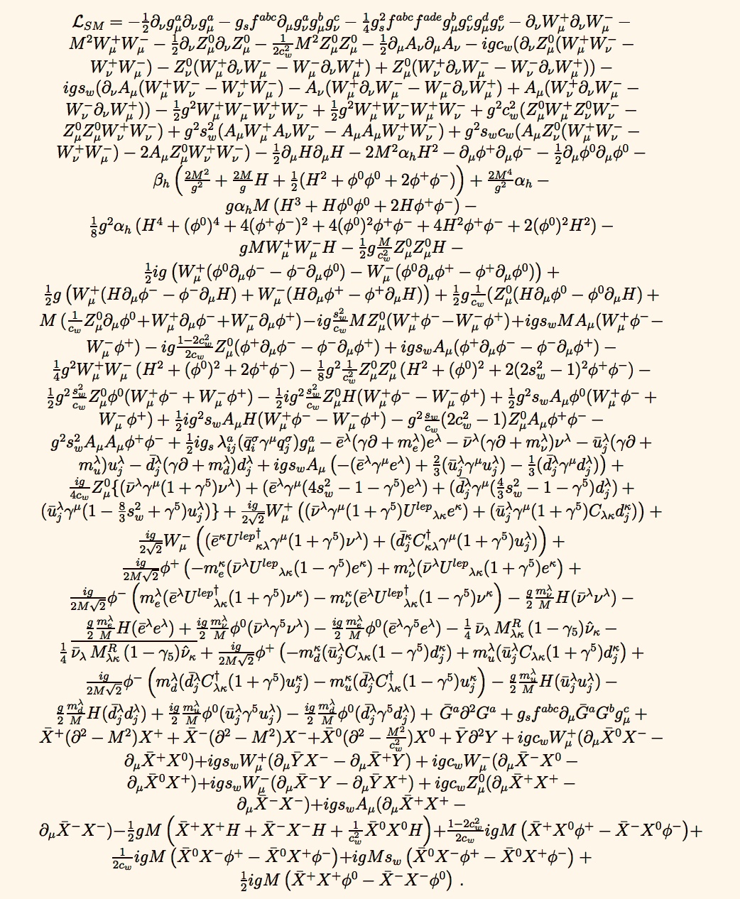
我们可以发现 Eular-Lagrange 方程非常适合进行坐标变换，或者说 Eular-Lagrange 方程具有坐标不变形（invariant）。后来人们发现很多物理定律，比如麦克斯韦的电磁理论、相对论等都可以囊括进 Eular-Lagrange 方程中，因此 Eular-Lagrange 方程更像一个经验规律，而最小作用量原理是一个在所有物理规律之上的更为广泛的规律，并且目前还没有反例。甚至是在粒子物理的研究中，第一步就是写出粒子的拉氏量。

下面是粒子物理标准模型（Standard Model）的拉氏量 \(\mathcal{L}_{SM}\) ，比较适合印在 T-shirt 上装逼。

Symmetry and Conservation

无限小的量是这样的一个量，它并不是零，所以我们不可以忽略它，但它确实又非常小，所以我们可以忽略所有它的平方等等。从这一节开始教授引入了广义坐标的概念，Euler-Lagrange 方程为

\[\frac{\mathrm{d}}{\mathrm{d}t}\frac{\partial\mathcal{L}}{\partial\dot{\boldsymbol{q}}}=\frac{\partial\mathcal{L}}{\partial\boldsymbol{q}}\\ \frac{\mathrm{d}}{\mathrm{d}t}\boldsymbol{p}=\frac{\partial\mathcal{L}}{\partial\boldsymbol{q}}\]

而 \(\boldsymbol{p}\) 称为 \(\boldsymbol{q}\) 的共轭动量（conjugate momentum），或者写成不同坐标分量的形式 \(\dot{p}_i=\partial\mathcal{L}/\partial q_i\) 亦可。

下面是一点守恒律的内容。考虑一个这样的系统，它的拉氏量如上，当 \(a=1\) 且 \(b=-1\) 的时候也就相当于系统的势能取决于 \(q_1-q_2\) 相对位置，这也是实际研究中很常见的情况。

\[\mathcal{L}=\frac{q_1^2+q_2^2}{2}-V(aq_1+bq_2)\]

经过不复杂的推导，有下面的守恒律存在

\[\frac{\mathrm{d}}{\mathrm{d}t}[b\dot{p}_1-a\dot{p}_2]=0\]

下面是一点对称性的内容。考虑一个依赖一个坐标的系统，其拉氏量为 \(\mathcal{L}=\dot{q}^2/2\) 现在做一个坐标变换（coordinate transformations）\(q^\prime=q+\delta\) ，这里的 \(\delta\) 不一定是一个小量只是一个固定的常数，这时我们必然有 \(\delta\mathcal{L}=0\) ，这就是对称性，更准确的说是空间平移对称性（translation symmetry），这个拉氏量在平移的操作下拉氏量的形式不发生变化。这样的平移对称性如果体现在上面的那个系统中，就相当于如果 \(q_1^\prime=q_1+b\delta\) 而 \(q_2^\prime=q_2-a\delta\) 坐标变换，那么就有 \(\delta\mathcal{L}=0\) 存在。

其它的对称性比如旋转对称性（rotational symmetry）。Susskind 在讨论旋转对称性的时候在笛卡尔坐标系下进行的操作，其实在极坐标下操作是更方便的。旋转对称性对应的是角动量守恒。

对称性和守恒律确实是成双成对出现的。假设坐标及其导数的变化量如下

\[\delta q_i=f_i(\boldsymbol{q})\delta\\ \delta\dot{q}_i=\dot{f_i}(\boldsymbol{q})\delta\]

那么拉氏量的变化量为

\[\begin{aligned} \delta\mathcal{L}&=\sum_i\frac{\partial\mathcal{L}}{\partial q_i}\delta q_i+\frac{\partial\mathcal{L}}{\partial\dot{q}_i}\delta\dot{q}_i =\sum_i\frac{\mathrm{d}}{\mathrm{d}t}\frac{\partial\mathcal{L}}{\partial \dot{q}_i}\delta q_i+p_i\delta\dot{q}_i\\ &=\sum_i\dot{p}_i\delta q_i+p_i\delta\dot{q}_i =\frac{\mathrm{d}}{\mathrm{d}t}\sum_ip_i\delta q_i \end{aligned} \]

如果这样的坐标变换存在对称性，那么 \(\delta\mathcal{L}=0\) 成立，这时有

\[\begin{aligned}\frac{\mathrm{d}}{\mathrm{d}t}\sum_ip_i\delta q_i&=0\\ \frac{\mathrm{d}}{\mathrm{d}t}\sum_ip_if_i(\boldsymbol{q})&=0\\ \sum_ip_if_i(\boldsymbol{q})&=\mathrm{const.} \end{aligned} \]

一定有一个对应的守恒律，我们将这个守恒量记为 \(\mathcal Q=\sum_ip_if_i(\boldsymbol{q})\) 。

需要注意的是，到目前为止我们还没有涉及到时间依赖的拉氏量，因此在对称性和守恒律中也不会出现时间这个量。我们没有讨论过能量守恒，能量守恒与上述的动量（广义动量）守恒有一点区别。动量守恒与空间对称性相关，而能量守恒与时间对称性相关。

另外物理中存在很多其它类型的对称性，比如镜像对称性等和这里说的对称性是不一样的，它们没有与之对应的守恒律。因为对于镜像对称性有 \(q\rightarrow -q\) 这样的坐标变换的对称，但是这样的对称性并不是累积起来的，考虑对称性的时候应当 \(q\rightarrow q+\delta\) 并且 \(\delta\) 是一个小量。

当然拉氏量不可能永远像之前描述得一样简单，只包含动能项（以下公式中的 quadratic term in velocity）和势能项，可能还包括如下式第三项的这样的耦合项

\[\mathcal{L}=\sum_{ij}T(\boldsymbol q)\dot{q_i}\dot{q_j}-V(\boldsymbol q)+\dot{q}f(\boldsymbol q)+\cdots\]

Hamiltonian

哈密顿量是能量的更深层次的概念（deeper concept of energy）。

系统的时间平移不变性（time translation invariance）就意味着能量守恒。如果一个系统的拉氏量 \(\mathcal{L}(q,\dot{q},t)\) 的表达式不显含时间 \(\mathcal{L}(q,\dot{q})\) ，只隐含时间（该系统的拉氏量会随时间发生变化是因为 \(\dot{q}\) 和 \(q\) 是随时间变化），那么这个系统就有时间平移不变性。之前对称性的定义是 \(\delta\mathcal L=0\) ，但时间平移不变性并不是使 \(\delta\mathcal L= 0\) 。拉氏量对时间的导数为

\[\frac{\mathrm{d}}{\mathrm{d}t}\mathcal{L}(\boldsymbol{q},\dot{\boldsymbol{q}})=\sum_i\frac{\partial\mathcal{L}}{\partial q_i}\dot{q_i}+\frac{\partial\mathcal{L}}{\partial\dot{q_i}}\ddot{q_i} =\sum_i\dot{p_i}\dot{q_i}+p_i\ddot{q_i}=\sum_i\frac{\mathrm{d}}{\mathrm d t}p_i\dot q_i\\ \frac{\mathrm{d}\mathcal{L}}{\mathrm{d}t}-\frac{\mathrm{d}}{\mathrm d t}\sum_ip_i\dot q_i=0 \]

上式中可以明显看到有一个守恒量，哈密顿量定义如下

\[\mathcal{H}=\sum_ip_i\dot q_i-\mathcal L \]

如果拉氏量的形式为 \(\mathcal L=m\dot x^2/2-V(x)\) ，那么这个系统的哈密顿量为 \(\mathcal H=m\dot x^2/2+V(x)\) 也就是我们常说的能量 \(E\) 。如果拉氏量是显含时间的，那么

\[\frac{\mathrm{d}}{\mathrm{d}t}\mathcal{L}(\boldsymbol{q},\dot{\boldsymbol{q}})=\sum_i\frac{\partial\mathcal{L}}{\partial q_i}\dot{q_i}+\frac{\partial\mathcal{L}}{\partial\dot{q_i}}\ddot{q_i} =\sum_i\dot{p_i}\dot{q_i}+p_i\ddot{q_i}=\sum_i\frac{\mathrm{d}}{\mathrm d t}p_i\dot q_i+\color{red}{\frac{\partial\mathcal L}{\partial t}}\\ \frac{\mathrm{d}\mathcal{L}}{\mathrm{d}t}-\frac{\mathrm{d}}{\mathrm d t}\sum_ip_i\dot q_i=\color{red}{\frac{\partial\mathcal L}{\partial t}}\]

因此这个系统的能量是不守恒的

\[ \frac{\mathrm d\mathcal H}{\mathrm dt}=\color{red}{-\frac{\partial\mathcal L}{\partial t}}\]

哈密顿量在量子力学中是一个非常重要的量。

Hamilton’s equations

有关微分的一个定理，如果一个全微分可以写为 \(\delta F(x,y)=A\delta x + B\delta y\) 这样的形式，那么一定有

\[\frac{\partial F}{\partial p}=A\\ \frac{\partial F}{\partial q}=B\]

然后哈密顿方程组可以很方便得推导出来

\[ \begin{aligned} \delta\mathcal H&=\delta\sum_i p_i\dot q_i-\mathcal L(\boldsymbol{q},\dot{\boldsymbol{q}})\\ &=\sum p_i\delta q_i+\dot q_i\delta p_i-\frac{\partial\mathcal L}{\partial q_i}\delta q_i -\frac{\partial\mathcal L}{\partial \dot q_i}\delta \dot q_i\\ &=\sum\dot q_i\delta p_i-\dot p_i\delta q_i\end{aligned}\]

可以得到哈密顿方程组

\[\begin{aligned}\frac{\partial\mathcal H}{\partial p_i}&=\dot q_i\\ \frac{\partial\mathcal H}{\partial q_i}&=-\dot p_i \end{aligned} \]

Euler-Lagrange 方程和哈密顿方程组是等效的，但是哈密顿方程组是一阶的方程，而 Euler-Lagrange 方程是一个二阶方程。我们也可以从哈密顿方程直接推出能量守恒（略）。

因为哈密顿量是一个守恒量 \(\mathcal H(\boldsymbol p, \boldsymbol q)=E\) ，那么在 \((\boldsymbol p, \boldsymbol q)\) 构成的相空间中，如果有 \(N\) 个坐标，那么对应的相空间就有 \(2N\) 个维度，而因为确定了系统的能量 \(E\) ，因此这个系统在相空间中的轨迹应当被约束在一个 \(2N-1\) 维的表面上。

Liouville’s theorem

刘维尔定理讨论的是相空间中相点流动的特性（the flow in phase space），把 \((\dot{\boldsymbol p},\dot{\boldsymbol{q}})\) 看作是相空间的一个速度场（flow vector），类似于流体力学中的速度场。在流体力学中，如果一个流体具有不可压缩（incompressible）的性质，那么对应的速度场的散度为零

\[\nabla\cdot\boldsymbol v=0\]

相空间中流体的不可压缩性与物理定律的时间反演性质（reversibility）相联系，更加形象的讨论可以直接看 Susskind 教授的视频。由哈密顿方程组可以直接得到系统在相空间中的不可压缩性

\[ \begin{aligned} \frac{\partial v_p}{\partial p}+\frac{\partial v_q}{\partial q}=-\frac{\partial}{\partial p}\frac{\partial\mathcal H}{\partial q}+\frac{\partial}{\partial q}\frac{\partial\mathcal H}{\partial p}=0 \end{aligned}\]

因此可以想象，对于在相空间中的一团流体元，虽然在运动过程中会发生形变，但是它们的体积是不变的，这也就是不可压缩性。比如 damped harmonic oscillator 的哈密顿量（能量）就在逐渐减小，而其在相空间中就体现出可压缩的性质。

Possion brackets

Curly brackets

\[\left\{F(\boldsymbol{p,q}),G(\boldsymbol{p,q})\right\}=\sum_i\frac{\partial F}{\partial q}\frac{\partial G}{\partial p}-\frac{\partial F}{\partial p}\frac{\partial G}{\partial q}\]

For example, If \(G(\boldsymbol{p,q})\) is the Hamiltonian, then the Possion brackets of \(F\) with \(G\) is the time derivative of \(F\) — the change in \(F\) when you change the time in one unit \(\varepsilon\)

\[\left\{F,\mathcal H\right\}=\frac{\mathrm dF}{\mathrm dt}=\frac{\delta F}{\varepsilon}\]

Possion brackets is a kind of algebra and has its own rules such as

\[\begin{aligned}\left\{A,B\right\}&=-\left\{B,A\right\}\\ \left\{AB,C\right\}&=A\left\{B,C\right\}+\left\{A,C\right\}B\end{aligned}\]

And there are some special cases

\[\left\{q_i,q_j\right\}=\left\{p_i,p_j\right\}=0\\ \left\{q_i,p_j\right\}=\delta_{ij}\]

For every symmetry, we have a conservation law. We take that thing which is conserved, and we take the possion brackets with this thing, and that gives us the small changes when we make symmetry transformations. The generator for translation is momentum, the generator for time translation is the Hamiltionian, the generator for angular translation is angular momentum.

F is a function in phase space and G is for generator. G generates some symmetry. If G is conserved, the Possion brackets of G and Hamiltonian is zero.

\[\frac{\mathrm dG}{\mathrm dt}=\left\{G(\boldsymbol{p,q}),\mathcal H\right\}=-\left\{\mathcal H,G(\boldsymbol{p,q})\right\}=0\]

泊松括号只是一些 fancy symbols 而已，在处理角动量的时候非常方便，角动量在量子力学中是非常重要的物理量。

EM field

唉，这一部分不想写了。

More is different

摘自：人民大学的屈帅同学的作业

More is different.

Philip W. Anderson

对称性意味着守恒量，该守恒量的观测是受到尺度效应影响的。宏观对称性和微观对称性之间相互独立又相互影响。比如微观对称性就对应着微观尺度上的守恒量，在微观尺度上该守恒量观测影响显著，相应的对称性也就尤为重要。在宏观尺度上，微观量对观测的影响就不是那么显著了，甚至会出现自发对称性破缺，微观守恒量不再影响观测。

这样导致的必然结果就是，宏观系统的演化不严格遵守微观对称性，发生自发对称性破缺。对称性自然而然就有了适用范围，例如 E. Wigner 提出的宇称守恒定律（Parity conservation），就被证实在弱相互作用下由于空间反演对称性破缺，宇称不守恒。

诸如此类还有热力学演化破缺了时间反演对称性，生物大分子破缺了左旋右旋对称性。实际上正是由于对称性破缺，我们的世界才丰富多彩。

不同尺度的问题有着其独特的对称性和复杂性。有着不同的相对理论和相对规律。随着尺度的增加，对称性降低，复杂性升高。在这个过程中，衍生出不同的科学。不同科学之间相互独立又相互交叉，作者想表达量变引起质变，整体与部分之和不同，比如超导、反铁磁、铁电、液晶等新奇物理现象都是由对称性破缺导致的。

粒子物理学家的标准粒子模型和天体物理学家的相对论都是不同尺度上的科学，我们既不能用简单的费曼图描述天体运动，也不能简单地用相对论描述夸克之间的作用。

PS

其实当时学得头头是道的，现在也就剩下拉氏量这个概念印象比较深刻了，人类遗忘的速度真的是非常快。