Fundamentals of Radio Interferometry

Notes from 18th Synthesis Imaging Workshop 2022. Rick Perley’s lectures are fantastic!

• Fundamentals of Radio Interferometry
• Radio Interferometry – Advanced Topics
• Basic Radio Interferometry – Geometry

Most basic interferometer

Here we have two perfect sensors. Vector \(\bm b\) is baseline vector and \(\bm s\) is the source direction.

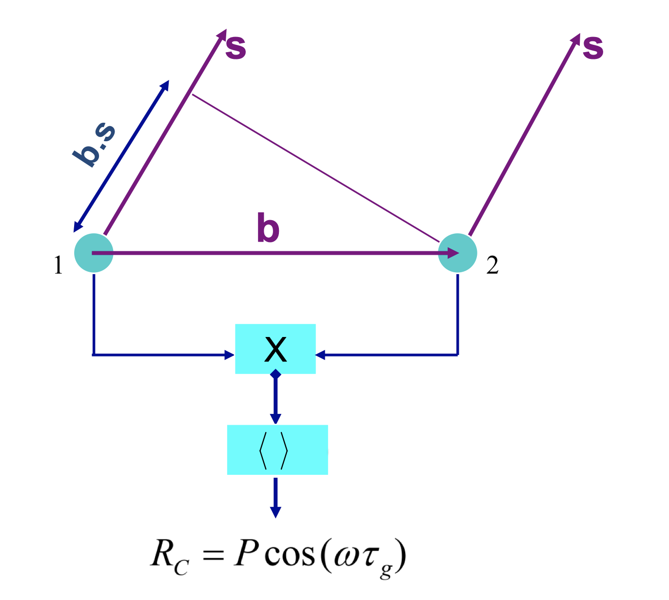
The geometric time delay is thus

\[\color{black}\tau_g=\bm b \cdot \bm s / c\]

which notes the time difference between these two sensors when light arrives. The sensor senses the Electric field and convert it to voltage variation.

\[\color{black}\begin{aligned} V_1&=E\cos[\omega(t-\tau_g)] \\ V_2&=E\cos(\omega t) \end{aligned}\]

Then these two signals enter into a correlator which does a simple multiplication

\[\color{black}V_1 V_2 = P[\cos(\omega \tau_g) + \cos(2\omega t - \omega\tau_g) ] \]

where \(\color{black}P\) is the power equals to \(\color{black}E^2/2\). It is clearly shown that the second term of the right hand side is a rapidly varying term while the first term is unchaning with time. The cosine response is then the time average of this multiplication

\[\color{black}R_c=P\cos(\omega\tau_g) \]

This response is only dependent on the geometric time delay. And if given the fixed length of baseline, \(\color{black}R_c\) only has an angle dependance. We can generate sine response by inserting a 90 degree phase shift in one of the signal paths.

\[\color{black}R_s=P\cos(\omega\tau_g) \]

It should be pointed out that the sensor doesn’t know where is the light coming from. The sensor retains the Electric fields from all directions. So the actual signal we would expect from the most basic inteferometer is an integral over the solid angle

\[\color{black}\begin{aligned} R_c&=\int I(\bm s)\cos(\omega\tau_g)\mathrm{d}\Omega \\ R_s&=\int I(\bm s)\sin(\omega\tau_g)\mathrm{d}\Omega \end{aligned}\]

where \(\color{black} R_c\) and \(\color{black} R_s\) record the even and odd components of the brightness function \(\color{black} I(\bm s)\) respectively. That is all we need to recover the brightness distribution on the sky.

Complex visibilities

Now we DEFINE the complex visibilites \(\color{black}V\) out of the independent real outputs \(\color{black} R_c\) and \(\color{black} R_s\) as

\[\color{blue}V_\nu(\bm{b})=R_c-iR_s=\int I_\nu(\bm s)e^{-2\pi i \nu\bm{b}\cdot\bm{s}/c}\mathrm{d}\Omega \]

where I replace the angular frequency \(\color{black} \omega\) with frequency \(\color{black}\nu\). A further simplication is to express the baseline vector as \(\color{black}(u\lambda, v\lambda)\), in the unit of wavelength and the source direction as direction cosines \(\color{black}(l,m)\), then we have

\[\color{green}V_\nu(u,v)\color{black}=\int I_\nu(l,m)e^{-2\pi i (ul+vm)}\mathrm{d}\Omega \]

More pratical

Include various pratical details.

Antenna response

\[\color{black}V_\nu(\bm{b})=\int \color{red}{A_1(\bm s)A_2^*(\bm s)}\color{black}I_\nu(\bm s)e^{-2\pi i \nu\bm{b}\cdot\bm{s}/c}\mathrm{d}\Omega \]

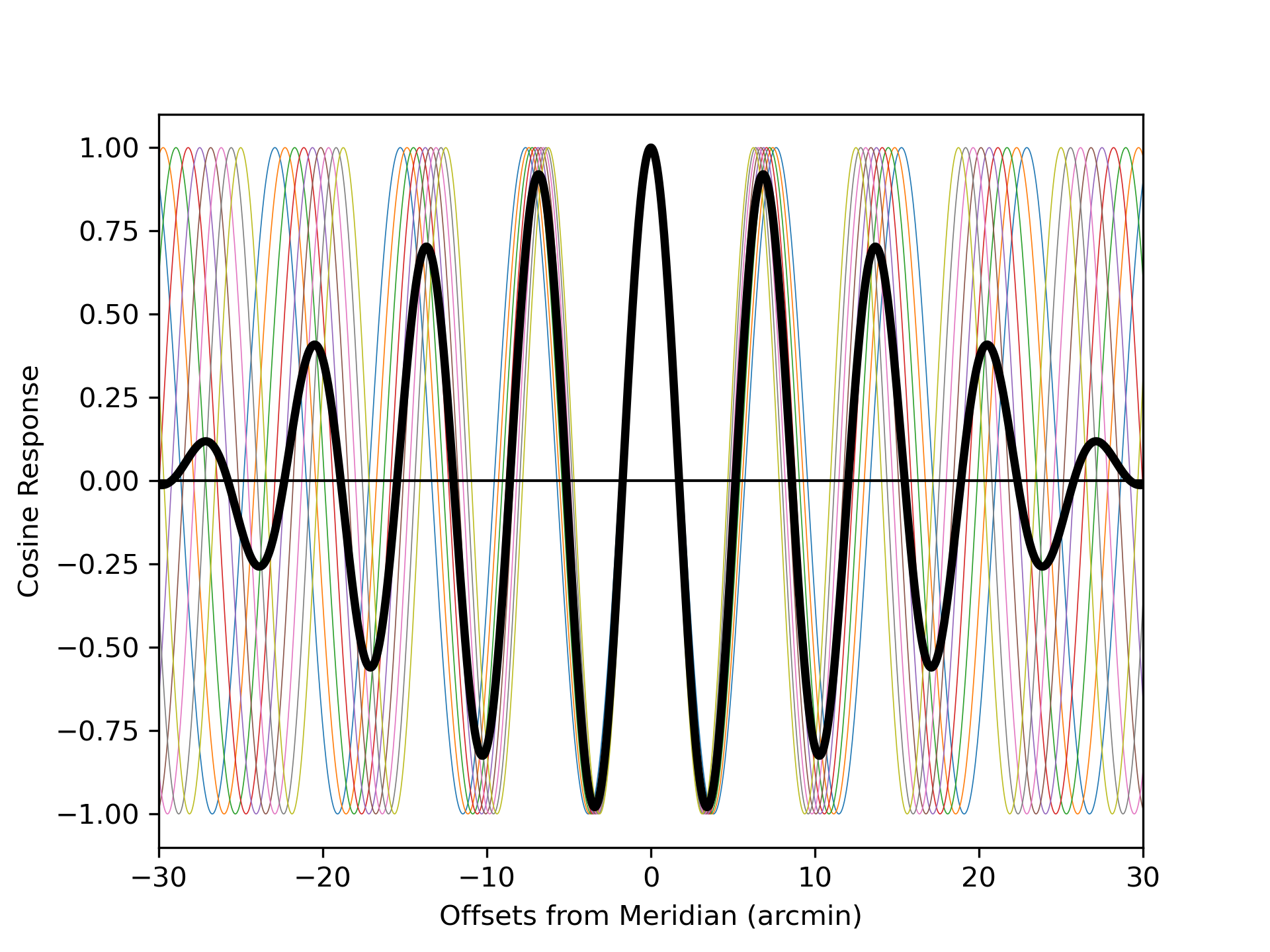
Finite Bandwidth

\[\color{black}V(\bm{b})=\int I_\nu(\bm s)\color{red}{\mathrm{sinc}(\tau_g\Delta\nu)}\color{black}e^{-2\pi i \nu_0\bm{b}\cdot\bm{s}/c}\mathrm{d}\Omega \]

You need delay tracking to track the source and keep it in between the two nulls in the fringe pattern.

finite_bw.py

x = np.linspace(-30,30,1000) # arcmin
us = np.linspace(450,550,3) # u = Baseline/Lambda

RC = lambda u: np.cos(2*np.pi*u*np.sin(x*np.pi/180/60)) # R_c = Pcos(2pi*ul)
RC_sum = 0.

fig, ax = plt.subplots()
for u in us:
    RCu = RC(u)
    ax.plot(x, RCu, lw=0.4)
    RC_sum += RCu

ax.plot(x, RC_sum/len(us), c='black', lw=3)
ax.hlines(0., x.min(), x.max(), color='black', lw=1)
ax.set_xlabel('Offsets from Meridian (arcmin)')
ax.set_ylabel('Cosine Response')
ax.set_xlim([x.min(), x.max()])

fig.show()

对任意一个基线来说，它只能在垂直与基线方向的那个方向获得最大的响应，也就是子午线上。因此对所有基线求和之后，只有天顶附近的一块很小的区域能获得比较高的响应，也就是所有基线子午线相交之处（忽略基线的三维分布）。

Source motion

The source is moving through the interferometer fringe pattern and the natural finge rate is about \(\color{black}v_f=u\omega_e\cos\delta\). Add phase shift to avoid the source from falling into the negative or zero response.

Finite time averaging

The reason is that the fringe tracking mechanism is correct for only one point in the sky. All others have a different rate.

对于 VLA 的 A configuration 来说，照相的积分时间不能超过 10 秒，这一点上和其它波段的观测区别很大，甚至是难以想象的，因为一般而言我们只要能够积分到足够多的时间，一个源的细节就越能被捕捉到。

Frequency Downconversion

High frequency components are much more expensive, and generally perform more poorly than low frequency components. Most radio interferometers use down conversion to translate the radio frequency information from the ‘RF’ to a lower frequency band.

Geometry

2-D Interferometers

Interferometers of which the baselines lie on a plane over time (earth rotation), for example all E-W interferometers or any 2-D array at a single instance of time can use the 2-D geometry. In both of these scenarios, accurate 2-D Fourier transform could be applied.

\[ \color{black} I_\nu(l,m)=\int V_\nu(u,v)e^{2\pi i (ul+vm)} \mathrm{d}u\mathrm{d}v \]

Imaging does this inversion.

3-D Interferometers

The complete relation between the visibility and sky brightness is now more complicated.

\[\color{black} V_\nu(u,v,w)=\int I_\nu(l,m)e^{-2\pi i (ul+vm+wn)}\mathrm{d}l\mathrm{d}m \]

💡Note that this is neither a 2-D or 3-D Fourier transform.
If we introduce phase tracking such that the phases are adjusted by \(e^{2\pi i w}\) and remembering that \(\color{black}l^2+m^2+n^2=1 \) we get

\[\color{black}V_\nu(u,v,w)=\int I_\nu(l,m)e^{-2\pi i[ul+vm+w(\sqrt{1-l^2-m^2}-1)]}\mathrm{d}l\mathrm{d}m\]

If the term \(\color{black}w(\sqrt{1-l^2-m^2}-1)\ll1\) is very small, then we can ignore it and return to a nice 2-D Fourier transform. Noting that \(\color{black}w<b/\lambda\) as a coordinate component of baseline vector \(\color{black}\bm b\) and if \(\color{black}l^2+m^2=\theta^2\ll1 \), one can write the condition for effective coplanarity as

\[\color{black} \begin{aligned} \frac{b}{\lambda}(1-\sqrt{1-\theta^2})&\ll1 \\ 1-\sqrt{1-\theta^2}&\ll\frac{\lambda}{b} \\ \frac{1}{2}\theta^2&\ll\frac{\lambda}{b} \\ \theta_\mathrm{max}&\ll\sqrt{2\theta_\mathrm{syn}} \end{aligned} \]

where \(\color{black} \theta_\mathrm{syn}\) is defined as the angular seperation between lobs \(\color{black}\lambda/b\). The above relation means that the main lob should include the FOV very well such we can approximate the 3-D interferometer to a 2-D one.

A further approximation is \(\color{black}\theta_\mathrm{max}\sim\lambda/D \) – the maximum angle for imaging is limited by the primary beam. Then we get the criterion

\[\color{black}\frac{\lambda b}{D^2}>1 \]

UV coverage

Each base line traces out an ellipse in UV plane over 24 hours

\[\color{black} u^2 + \left( \frac{v-B_z\cos\delta_0}{\sin\delta_0} \right)^2=B_y^2+B_z^2 \]