Imaging and Mosaicking

• Imaging Basics
• Mosaicking

每一次重温傅里叶变换都有新的认识！

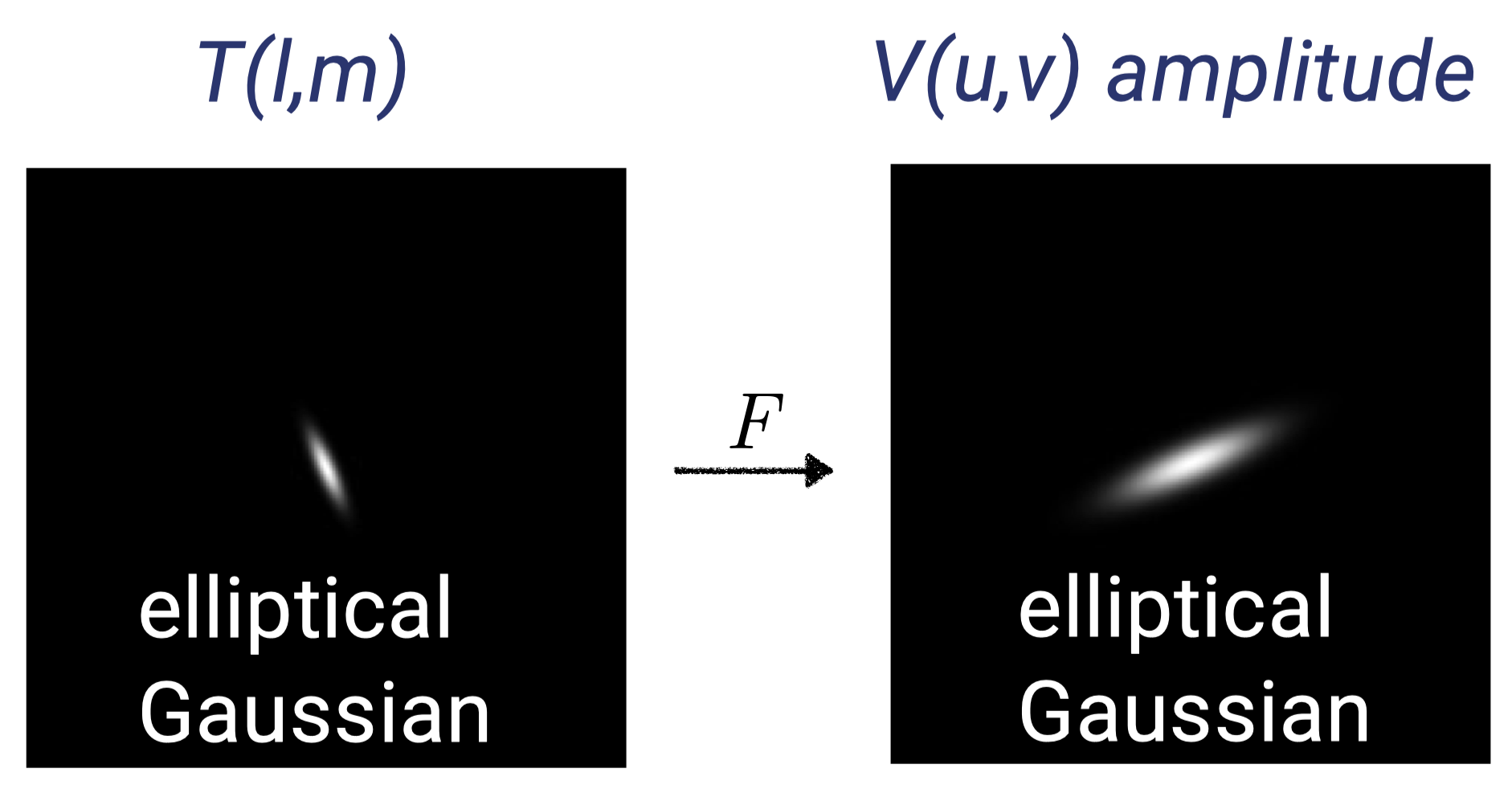
An offset in one domain is a phase shift in the other. \(\color{black}F(x)\) and \(\color{black}\tilde{F}(k)\) are Fourier pairs then

\[\color{black}F(x-x_0)=\tilde{F}(k)e^{i2\pi x_0k}\]

换句话说，源的位置移动反应在傅里叶空间是一个相位的变化，也就是相位决定了位置。

If we have now the calibrated visibilities, we can analyze the visibilities directly by model fitting on condition that the source has simple structures. Or to choose to recover an image from incomplete, nosiy samples of visibilities.

Imaging

Dirty Beam & Dirty Images

Visibilities data \(\color{black}V(u,v)\) is actually sampled by

\[\color{black}S(u,v)=\sum_{k=1}^{M}\delta(u-u_k,v-v_k)\]

The direct Fourier transform of visibilities is a dirty image

\[\color{black}V(u,v)S(u,v)\rightarrow T^D(l,m)\]

\[\color{black}T(l,m)*s(l,m)=T^D(l,m)\]

where the Fourier transform of the sampling pattern \(\color{black}s(l,m)\rightarrow S(u,v)\) is the point spread function or the synthesized beam. The dirty image is the true image convolved with the dirty beam.

Gridding

FFT is a must but it requires data on a regulary spaced grid. Conventional approach is to use convolution:

\[\color{black}V^G(u,v) = V(u,v)S(u,v) * G(u,v) \rightarrow T^D(l,m)g(l,m)\]

Now we can get our dirty image pretty fast.

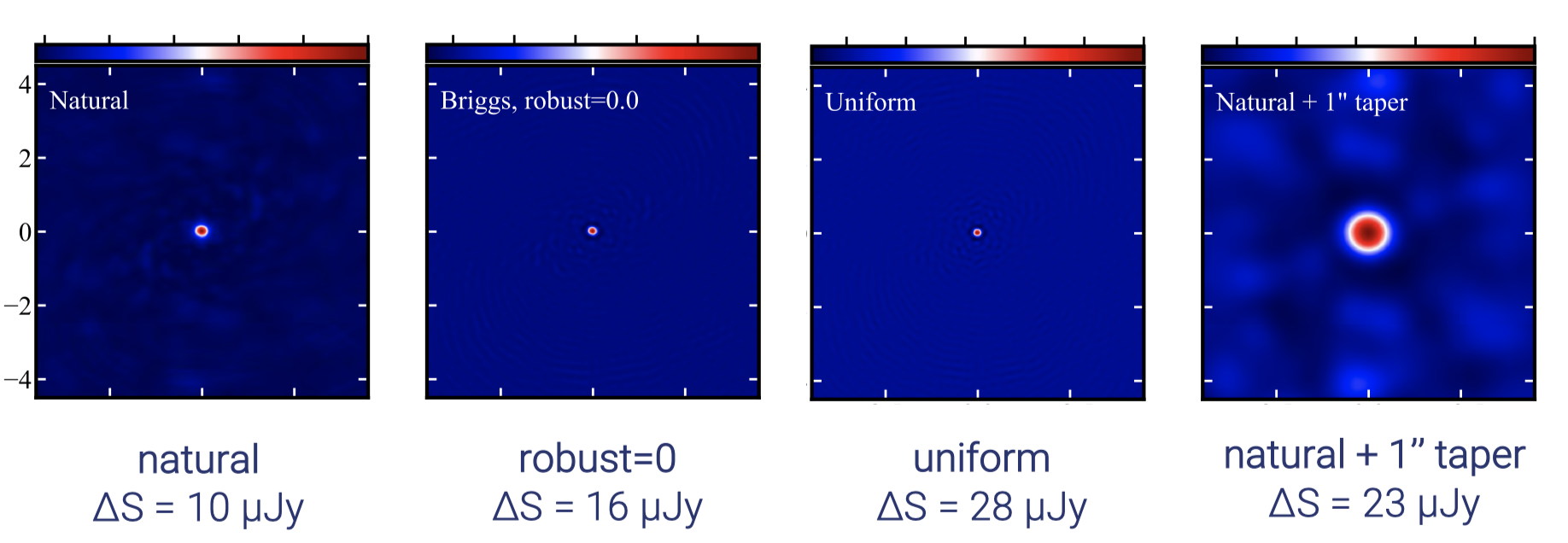
Weighting

Introduce weighting function \(\color{black}W(u,v)\) into the gridding process, this modifies the sampling function as \(\color{black}S(u,v)W(u,v)\) and changes the dirty beam shape \(\color{black}s(l,m)\). CASA uses Robust (Briggs) weighting that can usually obtain most of the natural weight sensitivity at the same time as most of uniform weight resolution.

The above sections will provide us dirty beam and dirty images. The next step is to clean the dirty images.

Deconvolution

Use non-linear techniques to interpolate/extrapolate \(\color{black}v(u,v)\) samples into unsampled regions of \(\color{black}(u,v)\) plane to find a plausible model of \(\color{black}T(l,m)\). A prior assumption about \(\color{black}T(l,m)\) is that it can be represented by point sources.

The dominant deconvolution algorithm in radio astronomy is CLEAN.

Classic Hogbom CLEAN algorithm

See Video Lecture 51:40 which has a vivid illustration.

Mosaicking

Pass.