VLA Continuum Tutorial 3C391

VLA Continuum Tutorial 3C391-CASA5.5.0

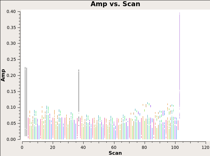
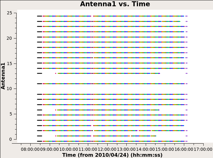
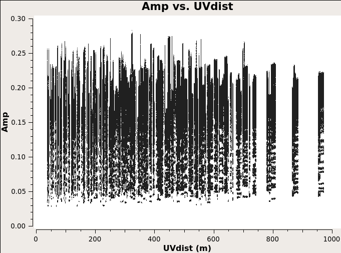
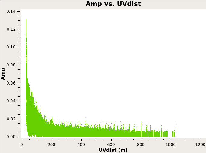
After flagging the data.

Examining the data

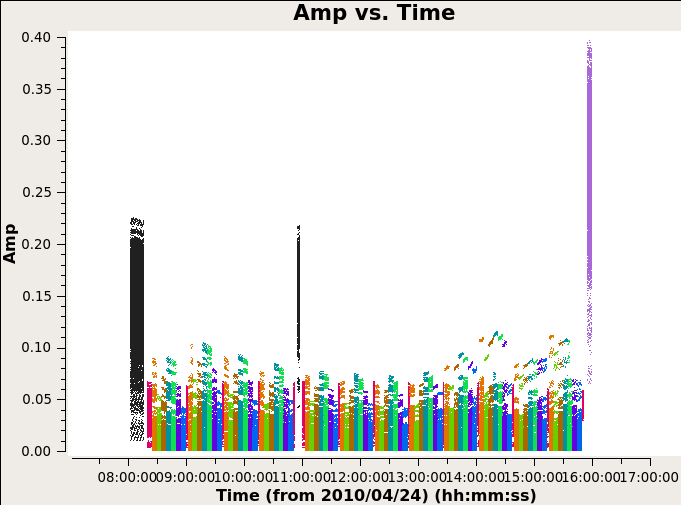
Below we can see the flagging process has taken effect.

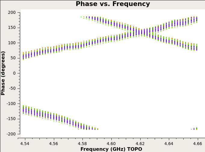
The phase \(\color{black}\theta=2\pi f \bm{b}\cdot\bm{s}/c\) is linearly dependent on frequency and the slope is \(\color{black}2\pi\bm{b}\cdot\bm{s}/c\). If we set iteraxis=baseline in plotms function, by clicking on the green arrow Next button we can switch the plots between different baselines and we will see that different baselines have different slopes.

Reference Antenna

Phase solutions are typically referred to a specific antenna. Phase corresponds to position. What we need is actually to align all the source positions to one point and it doesn’t matter where the point is.

Often we require the antenna be available over the entire observation. And in general, for calibration purposes, we would like to select an antenna that is close to the center of the array (but why?).

Use plotant to show the antenna positions.

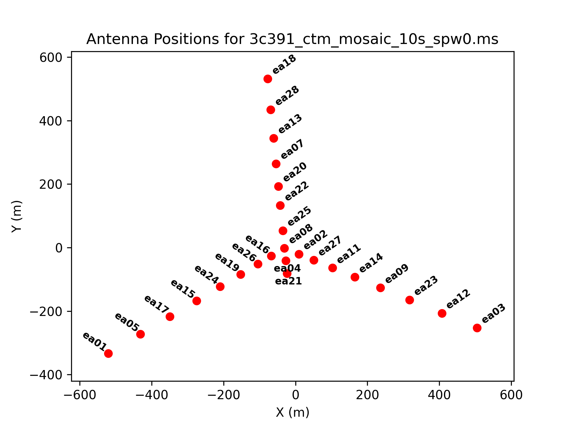
We will use antenna ea21 as the ref antenna later on.

Calibrating the Data

The calibration process in the tutorial is a bit different from the calibration lecture in the workshop. The observed visibility function is related to the true visibility by

\[\color{black}V_{ij}^\prime=b_{ij}(t)B_i(f,t)B_j^*(f,t)g_i(t)g_j(t)e^{i[\theta_i(t)-\theta_j(t)]}V_{ij}\]

In CASA the task gencal can specify calibration values of various types providing a means of antenna-based calibration values mannually.

Antenna Position Corrections

Specify values for \(\color{black}b_{ij}(t)\).

Initial Flux Density Scaling

Use task setjy to place the model visibility amplitude for the flux density calibrator 3C 286. By comparison with the observed data, determine the \(\color{black}g_i\) values.

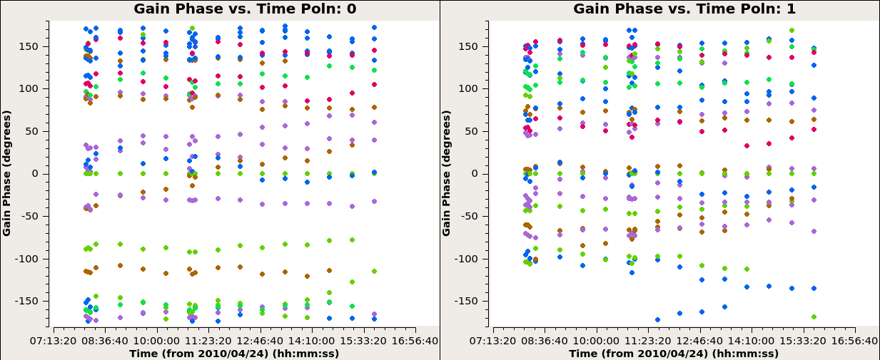
Initial Phase Calibration

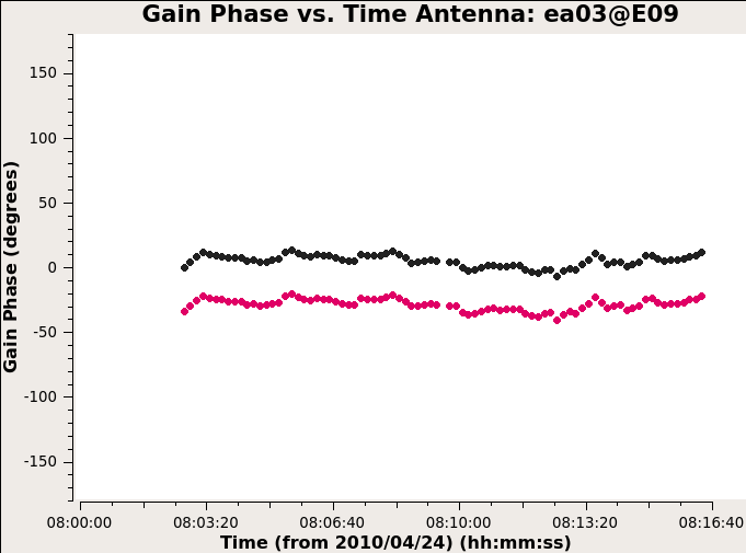
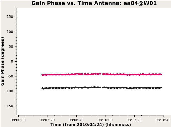
First we calculate the gain with task gaincal using all three calibrators to see if there are some bad data.

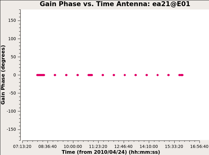
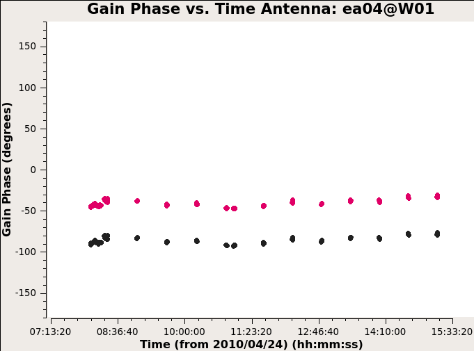
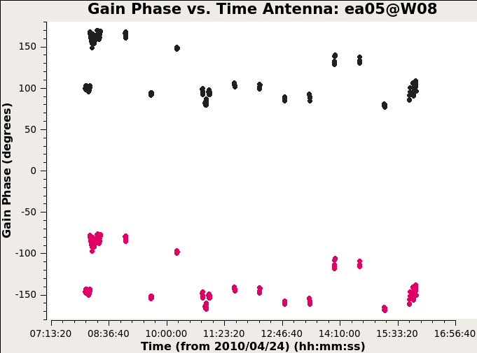
Antennas other than ea05 look OK so we flag it from the data. And again this time we use gaincal to calculate the gain using only the bandpass calibrator.

Still don’t completely understand this calibration step.

Delay Calibration

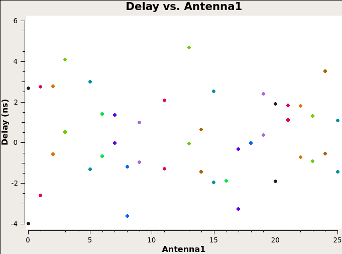
This step solves for the antenna-based delays (See Phase vs. Frequency plot above). Use gaincal with gaintype K to solve for the relative delay of each antenna relative to the reference antenna.

也就是说这里修正了不同天线的时间延迟，会让上面那一张 Phase vs. Frequency 的图里的曲线变成水平直线。

Bandpass Calibration

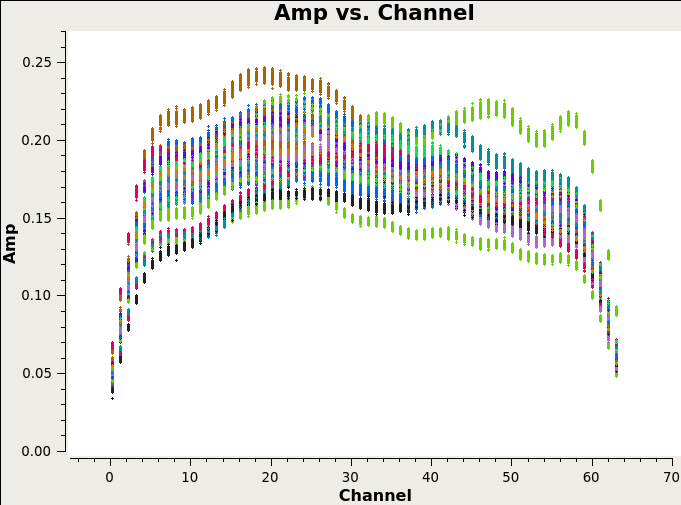
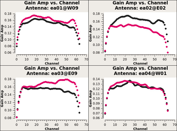
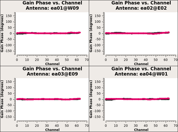
The task bandpass calculates the amplitude and phase as a function of frequency for each spectral window containing more than on channel. Correspondes to the complex bandpass \(\color{black}B_i(f,t)\).

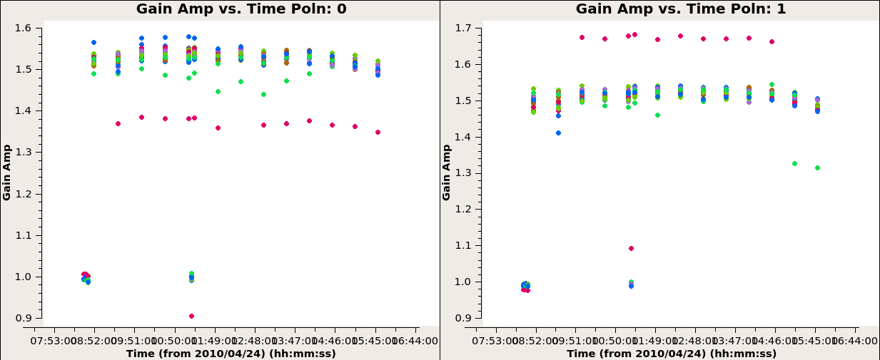
Gain Calibration

First, they use flux density calibrator 3C 286 to calculate the appropriate complex gains \(\color{black}g_i\) and \(\color{black}\theta_i\). Second, to minimize the differences through the atmosphere between the lines of sight to the gain calibrator 3C 286 and the target source, we also need to establish relative gain amplitudes and phases for different antennas using phase calibrator. The appropriate complex gains for a direction on the sky close to the target source will be determined from the phase calibrator.

已经开始看不明白了，就不能多写一点公式嘛！

Scaling the Amplitude Gains

我不理解。你为啥不理解？你要理解！真不理解。

Applying the Calibration

Use applycal to apply the calibration solutions to flux density calibrators J1331-3030(3C 286), visibility phase calibrator J1822-0938, target fields in the mosaic. Then we now have fully-calibrated visibilities in the CORRECTED-DATA column of the measurement set.

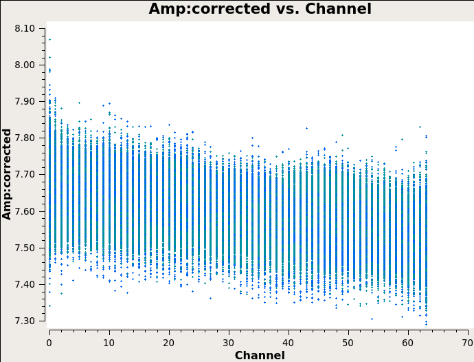
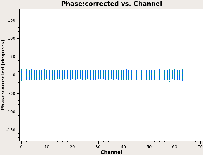
Then split off the target fields by split to create a new, calibrated measurement set containing all the target fields. After that, run statwt task to correct the data weights in the measurement set based on the variance of data.

总而言之，校准完毕！

Imaging

Examine the newly calibrated data.

Imaging parameters

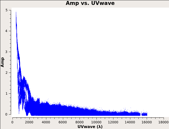
It is important to have an idea of what values to use for the image pixel (cell) size. The maximum baseline is about 16,000 wavelengths, i.e., the smallest angular scale of 12 arcseconds. The most effective cleaning occurs with at least 4-5 pixels across the synthesized beam. As such, we can chose the value of 2.5 arcseconds as the cell size.

Set the image size = [480,480] in this case to fully cover the supernova remnant and also take into account of FFT efficiency.

Multi-scale Mosaic Clean

Can’t believe this is not done automatically. I have to open a graphic viewer and select some clean regions mannually at the start of clean algorithm iterations.

Finally use viewer to show the cleaned image. In the DATA DISPLAY OPTIONS -> BASIC SETTINGS, I set the colormap to Hot Metal 2 and Scaling Power Cycles to -0.5. Here is what I get

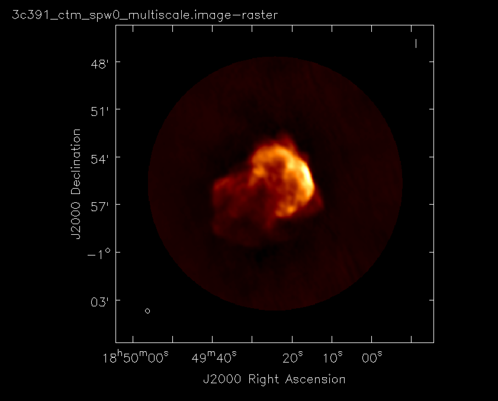
Image Analysis

Use CASA to determine the peak brightness, flux density and image noise level. Didn’t do this.