Magnification Matrix

对弱引力透镜效应中放大矩阵的介绍。

矩阵的特征值和特征向量

矩阵乘法就是线性变换，它的作用是旋转和拉伸一个向量，特征向量和特征值的定义

\[\color{black} A\boldsymbol{v}=\lambda \boldsymbol{v} \]

这是一个苍白的定义，应当注重它的意义，将矩阵进行特征分解

\[\color{black} A=Q\Lambda Q^{-1}\]

其中 \(\color{black} \Lambda\) 是对角阵，其对角元素为对应的特征值，\(\color{black} Q\) 矩阵的每一列是对应特征值的特征向量。下面我们以二维矩阵为例，选择单位特征向量，选取特殊的坐标系使得矩阵 \(\color{black}A\) 的其中一个特征向量和坐标轴重合，那么矩阵 \(\color{black}A\) 可以分解为

\[\color{black}A=\begin{bmatrix} 1 & \cos\theta \\ 0 & \sin\theta \end{bmatrix}\begin{bmatrix} \lambda_1 & 0 \\ 0 & \lambda_2 \end{bmatrix}\begin{bmatrix} 1 & -(\tan\theta)^{-1} \\ 0 & (\sin\theta)^{-1} \end{bmatrix}\]

\(\color{black}\lambda_1\) 和 \(\color{black}\lambda_2\) 这里我们设定都是正值，\(\color{black}\theta\) 是两个特征向量的夹角。接下来我将这个线性变换作用到任意一个向量上

\[\color{black}\begin{bmatrix} x^\prime \\ y^\prime \end{bmatrix}=\begin{bmatrix} \lambda_1 x + (\lambda_2-\lambda_1)(\tan\theta)^{-1}y \\ \lambda_2 y \end{bmatrix}\]

通过计算 \(\color{black} x^\prime/y^\prime\) 我们可以猜测它的方向变化

\[\color{black} \displaystyle{\frac{x^\prime}{y^\prime}={\displaystyle{\frac{\lambda_1}{\lambda_2}}\frac{x}{y}+\left(1-\frac{\lambda_1}{\lambda_2}\right)\frac{\cos\theta}{\sin\theta} }} \]

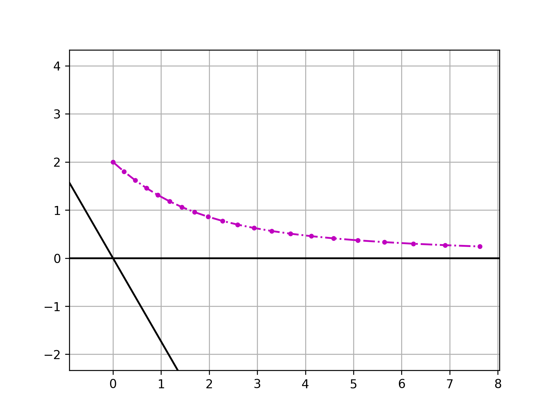
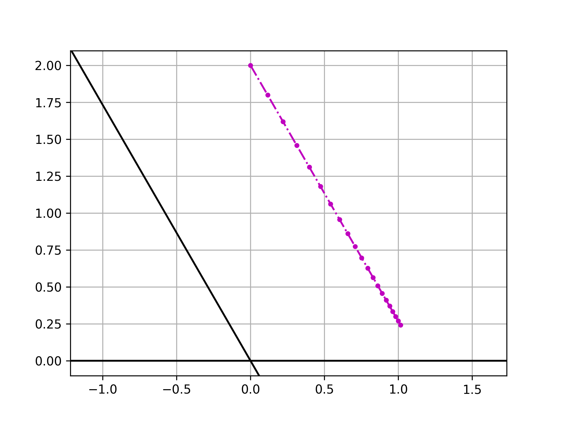
到这里还看不太出来，我们可以通过反复作用这个线性变换来看看所作用的向量的方向的变化，在作用 \(\color{black}n\) 次之后，向量方向变化为

\[\color{black} \frac{x^{(n)}}{y^{(n)}}=\left(\frac{\lambda_1}{\lambda_2}\right)^n \frac{x}{y}+\sum_{i=1}^{n}\left(\frac{\lambda_1}{\lambda_2}\right)^{n-1} \left(1-\frac{\lambda_1}{\lambda_2}\right)\frac{\cos\theta}{\sin\theta} \]

当 \(\color{black} \lambda_1 < \lambda_2\) 的时候，上式第一项趋于零，利用第二项和伯努利分布的相似性，我们可以知道第二项趋于 \(\color{black} \cos\theta/\sin\theta\)，因此在多次重复作用该线性变换之后，向量的方向会趋于 \(\color{black}\lambda_2\) 所对应的特征向量的方向。

\[\color{black}\lim_{n \to \infty}\sum_{i=1}^{n}\left(\frac{\lambda_1}{\lambda_2}\right)^{n-1} \left(1-\frac{\lambda_1}{\lambda_2}\right) = 1\]

因为我们总是可以选取一个坐标系使得其较大的特征值所对应的特征向量和坐标轴重合，所以如果 \(\color{black}\lambda_1>\lambda_2\)，那么该向量将向 \(\color{black}\lambda_1\) 所对应的特征向量上偏折。

而向量的长度，只有当主要的特征值 \(\color{black}\lambda_1=1\) 而另一个特征值 \(\color{black}\lambda_2<1\) 的时候，在不断进行同一个线性变换的时候，向量最终会趋于稳定。如果两个特征值都大于一，那么最后向量会不断拉伸；都小于一，那么向量的长度被不断压缩。

test.py

import numpy as np
import matplotlib.pyplot as plt

# parameters
theta = 120 * np.pi / 180
eigen_val = [1.1, 0.9]
eigen_vec = np.array([(1., 0.), (np.cos(theta), np.sin(theta))]).T
A = np.dot(eigen_vec,
    np.dot(np.diag(eigen_val), np.linalg.inv(eigen_vec)))

vec = np.array([[0.], [2.]])
for _ in range(20):
    vec = np.hstack([vec, np.dot(A, vec[:,-1]).reshape((2,1))])

# plot
fig, ax = plt.subplots()
ax.axhline(0., c='k')
ax.axline((0,0), (np.cos(theta), np.sin(theta)), c='k')
ax.plot(vec[0], vec[1], 'm.-.')
ax.axis('equal')
ax.grid('on')
plt.show()

矩阵的特征分解可以应用于图像压缩以及机器学习中的特征提取等领域。也可以将线性变换理解为向量运动的加速度，改变了向量的方向和大小。

矩阵的行列式和迹

「迹（trace）是矩阵在线性变换中留下的痕迹。」

矩阵的行列式和迹都是在相似变换下不变的量。矩阵的行列式和特征值的关系是

\[\color{black} \mathrm{det}(A)=\prod \lambda_i \]

它几何意义是体积的变化，在二维的情况下就是面积的变化，为证明它，我们考虑一个小的矢量面积元 \(\color{black}\mathrm{d}S = |\mathrm{d}\boldsymbol{x}\times\mathrm{d}\boldsymbol{y}| \)，经过矩阵 \(\color{black}A\) 的线性变换之后变为\(\color{black}\mathrm{d}S^\prime = |\mathrm{d}\boldsymbol{x}^\prime\times\mathrm{d}\boldsymbol{y}^\prime| \)，简单推导

\[\color{black} \begin{aligned} \mathrm{d}S^\prime &= |(A\mathrm{d}\boldsymbol{x})\times(A\mathrm{d}\boldsymbol{y})| \\ &= \left| \begin{bmatrix}A_{11}\mathrm{d}x_1+A_{12}\mathrm{d}x_2 \\ A_{21}\mathrm{d}x_1+A_{22}\mathrm{d}x_2 \end{bmatrix} \times\begin{bmatrix}A_{11}\mathrm{d}y_1+A_{12}\mathrm{d}y_2 \\ A_{21}\mathrm{d}y_1+A_{22}\mathrm{d}y_2 \end{bmatrix}\right| \\ &= |(A_{11}A_{22}-A_{12}A_{21})|\cdot|\mathrm{d}x_1\mathrm{d}y_2-\mathrm{d}x_2\mathrm{d}y_1| \\ &=|\mathrm{det}(A)|\cdot|\mathrm{d}\boldsymbol{x}\times\mathrm{d}\boldsymbol{y}| \\ &=|\mathrm{det}(A)|\mathrm{d}S \end{aligned}\]

下面考查一个特殊的矩阵 \(\color{black}A=I+P\)，其中 \(\color{black}P\) 是一个很小的扰动，即有 \(\color{black}P_{ij}\ll1\)，那么

\[\color{black}\begin{aligned} \mathrm{det}(A)&=\prod(1+P_{ii})+\mathcal{O}(P_{ij}^2)\\ &=1+\mathrm{tr}(P)+\mathcal{O}(P_{ij}^2)\end{aligned}\]

Magnification Matrix

Under thin lens approximation,

\[\color{black}A=\begin{pmatrix} 1-\partial_{11}\varphi & -\partial_{12}\varphi \\ -\partial_{12}\varphi & 1-\partial_{22}\varphi \end{pmatrix} \]

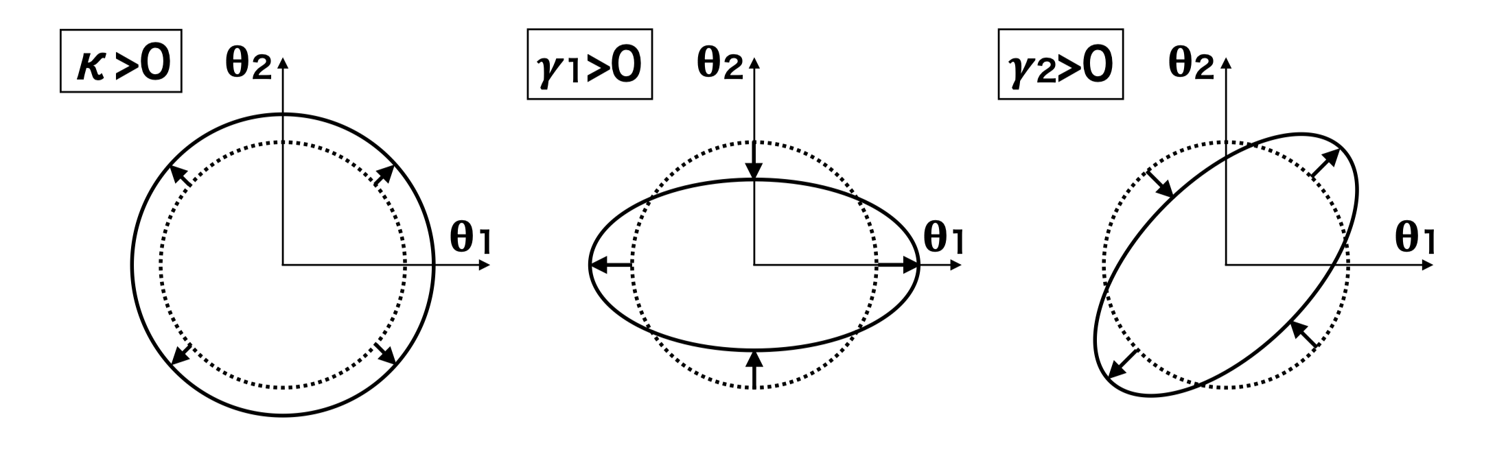
Manification matrix \(\color{black}A\) is the mapping matrix from image to source \(\color{black}\boldsymbol{\beta}=A\boldsymbol{\theta}\), the true position of the source is \(\color{black}\boldsymbol{\beta}\). Define convergence and shear

\[\color{black}\begin{aligned} \kappa&=\frac{1}{2}(\partial_{11}\varphi+\partial_{22}\varphi) \\ \gamma_1 &= \frac{1}{2}(\partial_{11}\varphi - \partial_{22}\varphi) \\ \gamma_2&=\partial_{12}\varphi \end{aligned}\]

Then the magnification matrix can be written as

\[\color{black}A=\begin{pmatrix} 1-\kappa-\gamma_1 & -\gamma_2 \\ -\gamma_2 & 1-\kappa+\gamma_1 \end{pmatrix} \]

The very first information about the matrix is the magnification of the image

\[\color{black}\mu=\mathrm{det}(A^{-1})=\frac{1}{\mathrm{det}(A)}=\frac{1}{(1-\kappa)^2+|\gamma|^2}\approx 1+2\kappa\]

where we have used the complex shear definition \(\color{black}\gamma=\gamma_1+i\gamma_2\). Then we can derive the eigenvalues of matrix \(\color{black}A\).

\[\color{black}\lambda=1-\kappa\pm|\gamma|\]

The inverse of the magnificaion matrix is a mapping from source to image

\[\color{black}A^{-1}=\mu\begin{pmatrix} 1-\kappa+\gamma_1 & \gamma_2 \\ \gamma_2 & 1-\kappa-\gamma_1 \end{pmatrix} \]

The corresponding eigenvalues are the inverse of eigenvalues of matrix \(\color{black}A\).

\[\color{black}\lambda=\frac{1}{1-\kappa\pm|\gamma|}\]

The direction angles of the eigenvectors are

\[\color{black}\tan\alpha=\frac{\gamma_2}{\gamma_1\mp|\gamma|}=\frac{-\gamma_1\mp|\gamma|}{\gamma_2}\]

Then if \(\color{black}\gamma_1=0\), the \(\color{black}\alpha=\pm\pi/2\), and this means the image will be elongated along one of these two directions. And if \(\color{black}\gamma_2=0\), we have \(\color{black}\alpha=0\) or \(\color{black}\pi/2\). In both cases, the two eigenvectors are perpendicular to each other and this is not the special case. One can prove that the eigenvectors of magnification matrix \(\color{black}A\) are always perpendicular to each other.

Or we can think of this in another way. Complex shear is spin-2 field and can thus be denoted as \(\color{black}\gamma=|\gamma|e^{i2\alpha}\), called position angle. And you can easily prove that \(\tan\alpha\) satisfies the above equation.

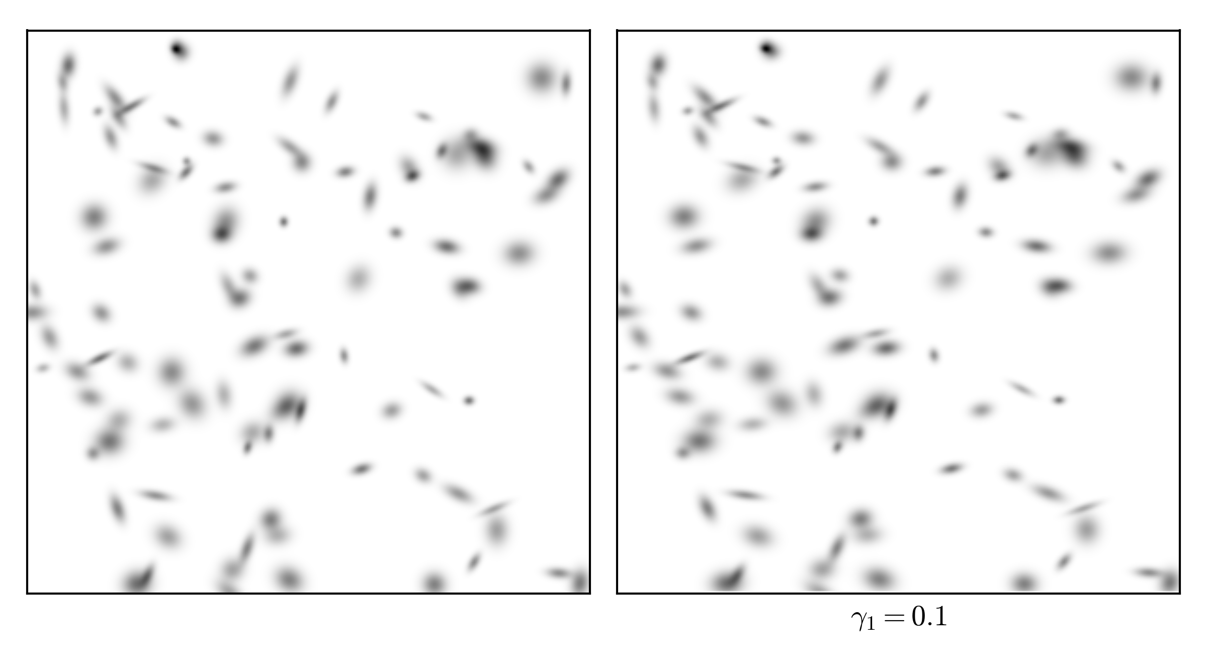
Shear effect on Gaussian source

One source

I will use astropy.model.Gaussian2D (which has the position angle as input parameter) as the galaxy brightness profile and show the shear effect. One would expect a \(\gamma=0.1\) shear effect from a galaxy cluster.

The source code to generate the above figures.

test.py

import numpy as np
from time import time
from astropy.modeling import models
import astropy.units as u
# scipy.interp2d is deprecated
from scipy.interpolate import LinearNDInterpolator
import matplotlib.pyplot as plt

imshape = (300, 300)
x_mean = imshape[1]//2
y_mean = imshape[0]//2
x, y = np.indices(imshape)
x -= x_mean # To keep the image galaxy in the center of field
y -= y_mean
pixlen = 0.03 # in arcsec

# Source galaxy shape information
x_stddev = 3.0 / 2.355 / pixlen
y_stddev = 2.0 / 2.355 / pixlen
theta = np.pi - 30. * np.pi / 180.
model = models.Gaussian2D(x_stddev=x_stddev, y_stddev=y_stddev, theta=theta)
source = model(x, y)

# Lensing Jacobin from source to image
A_g1_I = np.array(np.matrix([[1.-0.1, 0.0], [0.0, 1.+0.1]]).I)
A_g2_I = np.array(np.matrix([[1., -0.1], [-0.1, 1.]]).I)

# Image
def lens(source, A_I):
    A_I_x, A_I_y = np.dot(A_I, np.vstack([x.flatten(), y.flatten()]))
    image_interp = LinearNDInterpolator((A_I_x, A_I_y), source.flatten(), fill_value=0.)
    image = image_interp(x.T, y.T)
    return image
image_g1 = lens(source, A_g1_I)
image_g2 = lens(source, A_g2_I)

# Plot
plt.style.use('classic')
fig, ax = plt.subplots(nrows=1, ncols=3)
ax[0].imshow(source, cmap='gray_r', origin='lower')
ax[1].imshow(image_g1, cmap='gray_r', origin='lower')
ax[2].imshow(image_g2, cmap='gray_r', origin='lower')
ax[1].set_xlabel('$\gamma_1=0.1$', fontsize=14)
ax[2].set_xlabel('$\gamma_2=0.1$', fontsize=14)
for ax_i in ax:
    ax_i.set_xticks([])
    ax_i.set_yticks([])
plt.tight_layout()
plt.show()

One hundred sources

Here is the source code still using astropy.models.Gaussian2D. One can also use GalSim package to do this.

test.py

import numpy as np
from time import time
from astropy.modeling import models
import astropy.units as u
from scipy.interpolate import LinearNDInterpolator
import matplotlib.pyplot as plt

imshape = (300, 300)
pixlen = 0.3 # in arcsec

# Source models
rng = np.random.default_rng(1997)
nsrc = 100
model_params = [
    dict(amplitude=rng.uniform(.5, 1),
         x_mean=rng.uniform(0, imshape[1] - 1),
         y_mean=rng.uniform(0, imshape[0] - 1),
         x_stddev=rng.uniform(1./2.355/pixlen, 4./2.355/pixlen),
         y_stddev=rng.uniform(1./2.355/pixlen, 4./2.355/pixlen),
         theta=rng.uniform(0, np.pi))
    for _ in range(nsrc)]

model_list = [models.Gaussian2D(**kwargs) for kwargs in model_params]
source = np.zeros(imshape)
for model in model_list:
    model.render(source)

# Image
def lens(source, A_I):
    A_I_x, A_I_y = np.dot(A_I, np.vstack([x.flatten(), y.flatten()]))
    image_interp = LinearNDInterpolator((A_I_x, A_I_y), source.flatten(),fill_value=0.)
    image = image_interp(x.T, y.T)
    return image

image = np.zeros(imshape)
for model in model_list: # wait for a few minutes here
    x, y = np.indices(imshape)
    source_gal = model(x, y)
    # Ignore the position shift caused by lensing
    x, y = x - model.x_mean, y - model.y_mean
    image_gal = lens(source_gal, A_I)
    image += image_gal

# Save for further analysis
np.savetxt('source.txt', source)
np.savetxt('image.txt', image)

# Plot
plt.style.use('classic')
fig, ax = plt.subplots(nrows=1, ncols=2)
ax[0].imshow(source, cmap='gray_r', origin='lower')
ax[1].imshow(image, cmap='gray_r', origin='lower')
ax[1].set_xlabel('$\gamma_1=0.1$', fontsize=14)
for ax_i in ax:
    ax_i.set_xticks([])
    ax_i.set_yticks([])
plt.tight_layout()
plt.show()

Fourier Transform

My personal interest. Take the source and image data in one hundred sources case we have saved above, Fourier transform that.

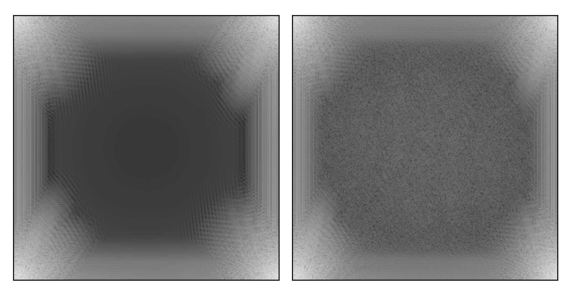
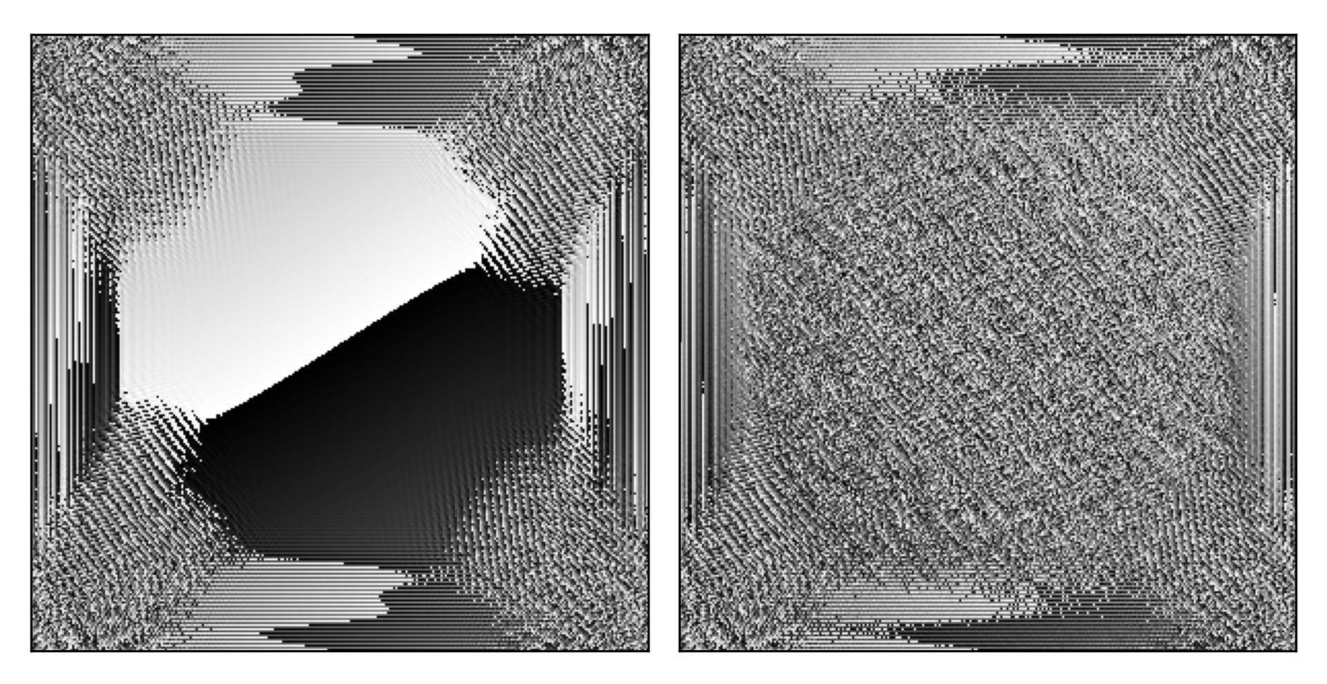
Not all Fourier transforms of images are meaningful. CMB is pure random field so its Fourier transforms are random fields as well and retain all the good statistical properties. In the case of galaxies, the coords are random, the source shapes are random, and it seems like adding them together would lead to something meaningless.

周期性的数据更适合傅里叶分析，并不是所有数据都适合傅里叶分析。